

Computing the speed of repayment of loans

1 - Introduction

Credit Risk refers to the likelihood that a borrower will not be able to repay a loan contracted by a lender. Thus throughout the years, financial institutions have developed various ways to quantify that risk so as to limit their exposure.

Here, instead of simply modeling whether a borrower will repay, by using Survival Analysis, it becomes possible to determine when this will happen. Indeed, it is easy to consider that fully repaying a loan is an explicit event, and therefore not having paid back the loan yet can be defined as the censored situation.

By using this configuration, banks, credit unions, or fintech startups in the lending space can predict the speed of repayment of a loan. This will help these institutions mitigate losses due to bad debt, customize interest rates, improve cash flow and credit collections, and determine which customers are likely to bring in the most revenue throughout a variety of products.

---

2 - Set up

In this tutorial, we will be using the German Credit dataset, which was originally provided by Professor Dr. Hans Hofmann of the University of Hamburg and available on the UCI Machine Learning Repository. The current version was adapted to be directly usable with a minimum amount of feature transformation..

3 - Dataset

3.1 - Overview

The dataset contains information useful to assess the borrowers creditworthiness as well as socio-demographic elements:

Feature category	Feature name	Type	Description
Time	duration	numerical	Duration in month
Event	full_repaid	categorical	Specifies if the loan was fully repaid
Socio-Demographic	age	numerical	Age of the borrower (in years)
Socio-Demographic	foreign_worker	numerical	Indicates if the borrower is a foreign worker
Socio-Demographic	personal_status	categorical	Gender and Marital status
Socio-Demographic	people_liable	numerical	Number of people being liable to provide maintenance for
Socio-Demographic	telephone	numerical	Indicates if the borrower owns a phone
Employment	employment_years	categorical	Years of employment at current job
Employment	job	categorical	Employment status
Residence	housing	categorical	Residential status of the borrower
Residence	present_residence	numerical	Years living at current residence
Loan information	amount	numerical	Amount of money borrowed
Loan information	installment_rate	numerical	Percentage of amount borrowed that will be charged by a lender to a borrower.
Loan information	purpose	categorical	Reason to get a loan
Bank information	checking_account_status	categorical	Status of the checking account
Bank information	credit_history	categorical	Credit history of the borrower
Bank information	number_of_credits	numerical	Number of existing credits at this bank
Bank information	other_installment_plans	categorical	Type of installments plans the borrower already has
Bank information	savings_account_status	categorical	Status of the saving account
Collateral/Guarantor	property	categorical	Type of valuable assets the borrower owns
Collateral/Guarantor	other_debtors	categorical	Indicate if someone else will be involved in the repayment or is guaranteeing the loan

# Importing modules
import pandas as pd
import numpy as np
from matplotlib import pyplot as plt
from pysurvival.datasets import Dataset
%pylab inline

# Reading the dataset
raw_dataset = Dataset('credit_risk').load()
print("The raw_dataset has the following shape: {}.".format(raw_dataset.shape))
raw_dataset.head(3)

Here is an overview of the raw dataset:

checking_account_status	duration	credit_history	...	foreign_worker	full_repaid
below_0	6	critical_account	...	1	1
0_to_200	48	existing_credit_paid	...	1	0
no_account	12	critical_account	...	1	1

3.2 - From categorical to numerical

There are several categorical features that need to encoded into one-hot vectors:

# From category to numerical
category_columns = [
    'checking_account_status', 'credit_history', 'purpose',
    'savings_account_status', 'employment_years', 'personal_status',
    'other_debtors', 'property', 'other_installment_plans', 'housing', 'job']
dataset = pd.get_dummies(raw_dataset, columns=category_columns, drop_first=True)

# Creating the time and event columns
time_column = 'duration'
event_column = 'full_repaid'

# Creating the features
features = np.setdiff1d(dataset.columns, [time_column, event_column] ).tolist()

---

4 - Exploratory Data Analysis

As this tutorial is mainly designed to provide an example of how to use PySurvival, we will not do a thorough exploratory data analysis here but greatly encourage the reader to do so by checking the predictive maintenance tutorial that provides a detailed analysis.

Here, we will just check if the dataset contains Null values or if it has duplicated rows. Then, we will take a look at feature correlations.

4.1 - Null values and duplicates

The first thing to do is checking if the raw_dataset contains Null values and has duplicated rows.

# Checking for null values
N_null = sum(dataset[features].isnull().sum())
print("The raw_dataset contains {} null values".format(N_null)) #0 null values

# Removing duplicates if there exist
N_dupli = sum(dataset.duplicated(keep='first'))
dataset = dataset.drop_duplicates(keep='first').reset_index(drop=True)
print("The raw_dataset contains {} duplicates".format(N_dupli))

# Number of samples in the dataset
N = dataset.shape[0]

As it turns out the raw_dataset doesn't have any Null values or duplicates.

4.2 - Correlations

Let's compute and visualize the correlation between the features

from pysurvival.utils.display import correlation_matrix
correlation_matrix(dataset[features], figure_size=(40,15), text_fontsize=7)

Figure 1 - Correlations

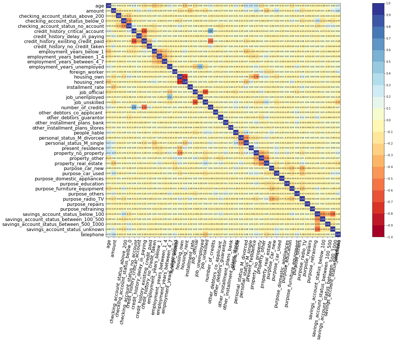
Based on the correlations chart, we should remove the following features

• credit_history_existing_credit_paid
• housing_own

to_remove = ['credit_history_existing_credit_paid', 'housing_own']
features = np.setdiff1d(features, to_remove).tolist()

---

5 - Modeling

So as to perform cross-validation later on and assess the performances of the model, let's split the dataset into training and testing sets.

# Building training and testing sets
from sklearn.model_selection import train_test_split
index_train, index_test = train_test_split( range(N), test_size = 0.4)
data_train = dataset.loc[index_train].reset_index( drop = True )
data_test  = dataset.loc[index_test].reset_index( drop = True )

# Creating the X, T and E inputs
X_train, X_test = data_train[features], data_test[features]
T_train, T_test = data_train[time_column], data_test[time_column]
E_train, E_test = data_train[event_column], data_test[event_column]

Let's now fit a Neural MTLR model to the training set.

Note: The choice of the structure of the neural network was obtained using grid-search hyperparameters selection, not displayed in this tutorial.

from pysurvival.models.multi_task import NeuralMultiTaskModel

# Initializing the Neural MTLR with a time axis split into 100 intervals
structure = [
                {'activation': 'ReLU', 'num_units': 60},
                {'activation': 'Swish', 'num_units': 60},
            ]
neural_mtlr = NeuralMultiTaskModel(bins=100, structure=structure)

# Fitting the model
neural_mtlr.fit(X_train, T_train, E_train,
                init_method = 'orthogonal', optimizer ='rprop', lr = 1e-4,
                l2_reg = 1e-1,  l2_smooth = 1e-1,
                batch_normalization = True,  bn_and_dropout = True,
                dropout=0.5,  num_epochs = 500)

We can take a look at the values of N-MTLR loss function to ensure that the fitting isn't incomplete

from pysurvival.utils.display import display_loss_values
display_loss_values(neural_mtlr)

Figure 2 - Neural MTLR loss function values

---

6 - Cross Validation

In order to assess the model performance, we previously split the original dataset into training and testing sets, so that we can now compute its performance metrics on the testing set:

6.1 - C-index

The C-index represents the global assessment of the model discrimination power: this is the model’s ability to correctly provide a reliable ranking of the survival times based on the individual risk scores. In general, when the C-index is close to 1, the model has an almost perfect discriminatory power; but if it is close to 0.5, it has no ability to discriminate between low and high risk subjects.

from pysurvival.utils.metrics import concordance_index
c_index = concordance_index(neural_mtlr, X_test, T_test, E_test)
print('C-index: {:.2f}'.format(c_index)) #0.76

---

6.2 - Brier Score

The Brier score measures the average discrepancies between the status and the estimated probabilities at a given time. Thus, the lower the score (usually below 0.25), the better the predictive performance. To assess the overall error measure across multiple time points, the Integrated Brier Score (IBS) is usually computed as well.

from pysurvival.utils.display import integrated_brier_score
integrated_brier_score(neural_mtlr, X_test, T_test, E_test, t_max=100,
                       figure_size=(20, 6.5) ) #0.08

Figure 3 - Neural MTLR loss function values

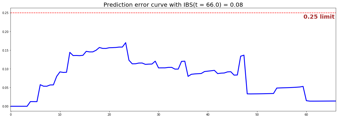
The IBS is equal to $0.08$ on the entire model time axis. This indicates that the model will have good predictive abilities.

---

7 - Predictions

7.1 - Overall predictions

Now that we have built a model that seems to provide great performances, let's compare the following:

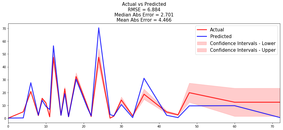
• the time series of the actual and predicted number of loans that were fully repaid, for each time t.

  from pysurvival.utils.display import compare_to_actual
  results = compare_to_actual(neural_mtlr, X_test, T_test, E_test,
                              is_at_risk = False,  figure_size=(16, 6),
                              metrics = ['rmse', 'mean', 'median'])
  

Figure 4 - Actual vs Predicted - Number of loans that were fully repaid

• the time series of the actual and predicted number of loans that were still active, for each time t.

  results = compare_to_actual(neural_mtlr, X_test, T_test, E_test,
                              is_at_risk = True,  figure_size=(16, 6),
                              metrics = ['rmse', 'mean', 'median'])
  

Figure 5 - Actual vs Predicted - Number of loans that were still active

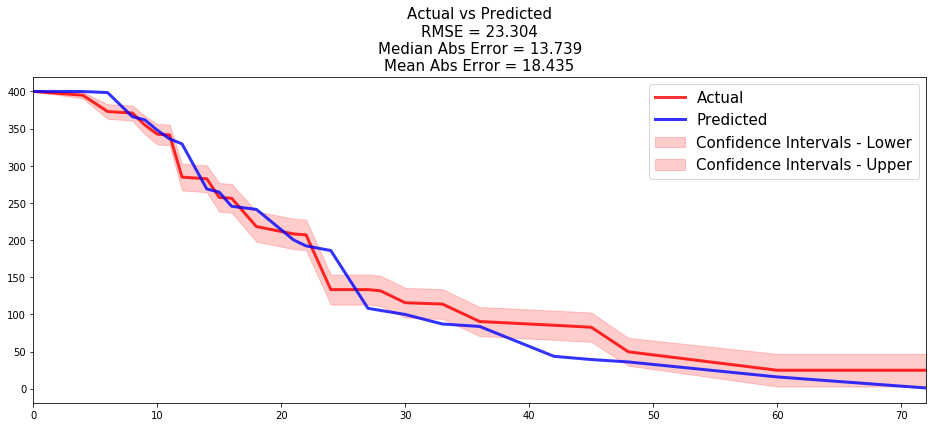
Both comparisons show that the model do a great job predicting the number of loans that were fully repaid (average absolute error of 4.5 loan) or that were still active (average absolute error of 18.4 loans) for all times t of the 70+ months time window.

---

7.2 - Individual predictions

Now that we know that we can provide reliable predictions for an entire cohort, let's compute the speed of repayment at the individual level. The speed of repayment is given by $\text{Speed}(t) = 1 - \text{Survival}(t)$

First, we can construct the risk groups based on risk scores distribution. The helper function create_risk_groups, which can be found in pysurvival.utils, will help us do that:

from pysurvival.utils.display import create_risk_groups

risk_groups = create_risk_groups(model=neural_mtlr, X=X_test,
    use_log = True, num_bins=30, figure_size=(20, 4),
    low= {'lower_bound':0, 'upper_bound':1.64, 'color':'red'},
    medium= {'lower_bound': 1.64, 'upper_bound':1.8, 'color':'green'},
    high= {'lower_bound':1.8, 'upper_bound':3, 'color':'blue'}
    )

Figure 6 - Creating risk groups

Note: The current choice of the lower and upper bounds for each group is based on my intuition; so feel free to change the values so as to match your situation instead.

Here, it is possible to distinguish 3 main groups, low, medium and high risk groups. Because the C-index is high, the model will be able to rank the survival times of a random unit of each group, such that $t_{high} \leq t_{medium} \leq t_{low}$.

Let's randomly select individual unit in each group and compare their speed of repayment functions. To demonstrate our point, we will purposely select units which experienced an event to visualize the actual time of event.

# Initializing the figure
fig, ax = plt.subplots(figsize=(15, 5))

# Selecting a random individual that experienced an event from each group
groups = []
for i, (label, (color, indexes)) in enumerate(risk_groups.items()) :

    # Selecting the individuals that belong to this group
    if len(indexes) == 0 :
        continue
    X = X_test.values[indexes, :]
    T = T_test.values[indexes]
    E = E_test.values[indexes]

    # Randomly extracting an individual that experienced an event
    choices = np.argwhere((E==1.)).flatten()
    if len(choices) == 0 :
        continue
    k = np.random.choice( choices, 1)[0]

    # Saving the time of event
    t = T[k]

    # Computing the CDF for all times t
    cdf = 1. - neural_mtlr.predict_survival(X[k, :]).flatten()

    # Displaying the functions
    label_ = '{} risk'.format(label)
    plt.plot(neural_mtlr.times, cdf, color = color, label=label_, lw=2)
    groups.append(label)

    # Actual time
    plt.axvline(x=t, color=color, ls ='--')
    ax.annotate('T={:.1f}'.format(t), xy=(t, 0.5*(1.+0.2*i)),
        xytext=(t, 0.5*(1.+0.2*i)), fontsize=12)

# Show everything
groups_str = ', '.join(groups)
title = "Comparing cumulative density functions between {} risk grades"
title = title.format(groups_str)
plt.legend(fontsize=12)
plt.title(title, fontsize=15)
plt.xlim(0, 65)
plt.ylim(0, 1.05)
plt.show()

Figure 7 - Predicting individual speed of repayment functions

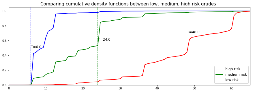
As we can see, the model manages to perfectly predict the event time, here it corresponds to a sudden increase in the individual speed of repayment function.

---

8 - Conclusion

We can now save our model so as to put it in production and score future borrowers.

# Let's now save our model
from pysurvival.utils import save_model
save_model(neural_mtlr, '/Users/xxx/Desktop/credit_neural_mtlr.zip')

Thanks to Survival Analysis, we can see that it is indeed possible to predict the speed of repayment of loans and forecast the number of loans that will be fully repaid throughout time, which is a great advantage over classification modeling.

---

References

• German Credit dataset - UCI Machine Learning Repository