Conditional Survival Forest model
The Conditional Survival Forest model was developed by Wright et al. in 2017 to improve the Random Survival Forest training, whose objective function tends to favor splitting variables with many possible split points.
Instance
To create an instance, use pysurvival.models.survival_forest.ConditionalSurvivalForestModel.
Attributes
max_features: str or int -- The number of features randomly chosen at each split.num_trees: int -- number of trees contained in the foresttimes: array-like -- representation of the time axis of the modeltime_buckets: array-like -- representation of the time axis of the model using time bins, which are represented byvariable_importance: dict -- importance of each feature (the higher, the more important the feature is). The importance is the difference between the perturbed and unperturbed error rate for each feature.
Methods
__init__ - Initialize the estimator
ConditionalSurvivalForestModel(num_trees = 10)
Parameters:
num_trees: int (default=10) -- number of trees that will be built in the forest.
fit - Fit the estimator based on the given parameters
fit(X, T, E, max_features = 'sqrt', max_depth = 5,
    min_node_size = 10, alpha = 0.05, minprop= 0.1, num_threads = -1,
    weights = None, sample_size_pct = 0.63,
    importance_mode = 'normalized_permutation',  seed = None,
    save_memory=False )
Parameters:
-
X: array-like -- input samples; where the rows correspond to an individual sample and the columns represent the features (shape=[n_samples, n_features]). -
T: array-like -- target values describing the time when the event of interest or censoring occurred. -
E: array-like -- values that indicate if the event of interest occurred i.e.: E[i]=1 corresponds to an event, and E[i] = 0 means censoring, for all i. -
max_features: int, float or string (default="sqrt") -- number of features to consider when looking for the best split:- If int, then consider the given value at each split.
- If float, then
max_featuresis a fraction andint(max_features * n_features)features are considered at each split. - If "sqrt", then
max_features=sqrt(n_features) - If "log2", then
max_features=log2(n_features). - If "all", then
max_features=n_features.
-
min_node_size: int (default=10) -- minimum number of samples required to be at a leaf node -
alpha: float (default=0.05) -- significance threshold to allow splitting. -
minprop: float (default=0.1) -- lower quantile of covariate distribution to be considered for splitting -
num_threads: int (default= -1) -- number of jobs to run in parallel during training. If -1, then the number of jobs is set to the total number of available cores. -
weights: array-like (default = None) -- weights for sampling of training observations. Observations with larger weights will be selected with higher probability in the bootstrap. The sum of the weights needs to be 1. -
sample_size_pct: double (default = 0.63) -- percentage of original samples used in each tree building -
importance_mode: str (default='impurity_corrected') -- variable importance mode. Here are the available options:impurityorimpurity_corrected: it's the unbiased heterogeneity reduction developed by Sandri & Zuccolotto (2008)permutationit's unnormalized as recommended by Nicodemus et al.normalized_permutationit's normalized version of the permutation importance computations by Breiman et al.
-
seed: int (default=None) -- seed used by the random number generator. If None, the current timestamp converted in UNIX is used. -
save_memory: bool (default=False) -- Use memory saving splitting mode. This will slow down the model training. So, only set toTrueif you encounter memory problems.
Returns:
self: object
predict_hazard - Predicts the hazard function
predict_hazard(x, t = None)
Parameters:
-
x: array-like -- input samples; where the rows correspond to an individual sample and the columns represent the features (shape=[n_samples, n_features]). -
t: double (default=None) -- time at which the prediction should be performed. If None, then return the function for all available t.
Returns:
hazard: numpy.ndarray -- array-like representing the prediction of the hazard function
predict_survival - Predicts the survival function
predict_survival(x, t = None)
Parameters:
-
x: array-like -- input samples; where the rows correspond to an individual sample and the columns represent the features (shape=[n_samples, n_features]). -
t: double (default=None) -- time at which the prediction should be performed. If None, then return the function for all available t.
Returns:
survival: numpy.ndarray -- array-like representing the prediction of the survival function
predict_risk - Predicts the risk score
predict_risk(x)
Parameters:
x: array-like -- input samples; where the rows correspond to an individual sample and the columns represent the features (shape=[n_samples, n_features]).
Returns:
risk_score: numpy.ndarray -- array-like representing the prediction of the risk score
Example
Let's now take a look at how to use the Conditional Survival Forest (CSF) model on a simulation dataset generated from a parametric model.
#### 1 - Importing packages
import numpy as np
import pandas as pd
from matplotlib import pyplot as plt
from sklearn.model_selection import train_test_split
from pysurvival.models.simulations import SimulationModel
from pysurvival.models.survival_forest import ConditionalSurvivalForestModel
from pysurvival.utils.metrics import concordance_index
from pysurvival.utils.display import integrated_brier_score
%pylab inline

#### 2 - Generating the dataset from a Exponential parametric model
# Initializing the simulation model
sim = SimulationModel( survival_distribution = 'exponential',
                       risk_type = 'linear',
                       censored_parameter = 1,
                       alpha = 3)

# Generating N random samples
N = 1000
dataset = sim.generate_data(num_samples = N, num_features=4)

# Showing a few data-points
dataset.head(2)
| x_1 | x_2 | x_3 | x_4 | time | event |
|---|---|---|---|---|---|
| 0.061498 | 7.065547 | 0.004457 | 0.131379 | 15.412209 | 0. |
| 0.079149 | 6.732271 | 0.008654 | 0.090398 | 0.000700 | 1. |
PySurvival also displays the Base Survival function of the Simulation model:
from pysurvival.utils.display import display_baseline_simulations
display_baseline_simulations(sim, figure_size=(20, 6))

#### 3 - Creating the modeling dataset
# Defining the features
features = sim.features

# Building training and testing sets #
index_train, index_test = train_test_split( range(N), test_size = 0.2)
data_train = dataset.loc[index_train].reset_index( drop = True )
data_test  = dataset.loc[index_test].reset_index( drop = True )

# Creating the X, T and E input
X_train, X_test = data_train[features], data_test[features]
T_train, T_test = data_train['time'].values, data_test['time'].values
E_train, E_test = data_train['event'].values, data_test['event'].values


#### 4 - Creating an instance of the Conditional model and fitting the data.
# Building the model
csf = ConditionalSurvivalForestModel(num_trees=200)
csf.fit(X_train, T_train, E_train,
        max_features="sqrt", max_depth=5, min_node_size=20,
        alpha = 0.05, minprop=0.1)


#### 5 - Cross Validation / Model Performances
c_index = concordance_index(csf, X_test, T_test, E_test) #0.81
print('C-index: {:.2f}'.format(c_index))

ibs = integrated_brier_score(csf, X_test, T_test, E_test, t_max=30,
            figure_size=(20, 6.5) )
print('IBS: {:.2f}'.format(ibs))
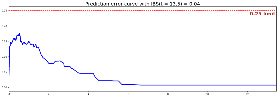
We can see that the c-index is well above 0.5 and that the Prediction error curve is below the 0.25 limit, thus the model yields great performances.

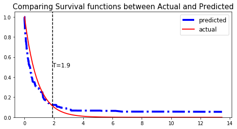
We can show this by randomly selecting datapoints and comparing the actual and predicted survival functions, computed by the simulation model and the CSF respectively.
# Initializing the figure
fig, ax = plt.subplots(figsize=(8, 4))

# Randomly extracting a data-point that experienced an event
choices = np.argwhere((E_test==1.)&(T_test>=1)).flatten()
k = np.random.choice( choices, 1)[0]

# Saving the time of event
t = T_test[k]

# Computing the Survival function for all times t
survival = csf.predict_survival(X_test.values[k, :]).flatten()
actual = sim.predict_survival(X_test.values[k, :]).flatten()

# Displaying the functions
plt.plot(csf.times, survival, color = 'blue', label='predicted', lw=4, ls = '-.')
plt.plot(sim.times, actual, color = 'red', label='actual', lw=2)

# Actual time
plt.axvline(x=t, color='black', ls ='--')
ax.annotate('T={:.1f}'.format(t), xy=(t, 0.5), xytext=(t, 0.5), fontsize=12)

# Show everything
title = "Comparing Survival functions between Actual and Predicted"
plt.legend(fontsize=12)
plt.title(title, fontsize=15)
plt.ylim(0, 1.05)
plt.show()
