Linear MTLR model
The Multi-Task Logistic Regression (MTLR) model is an alternative to the Cox’s proportional hazard model. It can be seen as a series of logistic regression models built on different time intervals so as to estimate the probability that the event of interest happened within each interval.
The model was introduced by Yu, Chun-Nam, et al. in 2011
Instance
To create an instance, use pysurvival.models.multi_task.LinearMultiTaskModel.
Attributes
times: array-like -- representation of the time axis of the modeltime_buckets: array-like -- representation of the time axis of the model using time bins, which are represented by
Methods
__init__ - Initialization
LinearMultiTaskModel(bins=100, auto_scaler=True)
Parameters:
bins: int (default=100) -- Number of subdivisions of the time axisauto_scaler: bool (default=True) -- Determines whether a sklearn scaler should be automatically applied
fit - Fit the estimator based on the given parameters
fit(X, T, E, init_method = 'glorot_uniform', optimizer ='adam',
    lr = 1e-4, num_epochs = 1000, l2_reg=1e-2, l2_smooth=1e-2,
    verbose=True, extra_pct_time = 0.1, is_min_time_zero=True)
Parameters:
-
X: array-like -- input samples; where the rows correspond to an individual sample and the columns represent the features (shape=[n_samples, n_features]). -
T: array-like -- target values describing the time when the event of interest or censoring occurred. -
E: array-like -- values that indicate if the event of interest occurred i.e.: E[i]=1 corresponds to an event, and E[i] = 0 means censoring, for all i. -
init_method: str (default = 'glorot_uniform') -- Initialization method to use. Here are the possible options:glorot_uniform: Glorot/Xavier uniform initializerhe_uniform: He uniform variance scaling initializeruniform: Initializing tensors with uniform (-1, 1) distributionglorot_normal: Glorot normal initializer,he_normal: He normal initializer.normal: Initializing tensors with standard normal distributionones: Initializing tensors to 1zeros: Initializing tensors to 0orthogonal: Initializing tensors with a orthogonal matrix,
-
optimizer: str (default = 'adam') -- iterative method for optimizing a differentiable objective function. Here are the possible options:adadeltaadagradadamadamaxrmspropsparseadamsgd
-
lr: float (default=1e-4) -- learning rate used in the optimization -
num_epochs: int (default=1000) -- number of iterations in the optimization -
l2_reg: float (default=1e-4) -- L2 regularization parameter for the model coefficients -
l2_smooth: float (default=1e-4) -- Second L2 regularizer that ensures the parameters vary smoothly across consecutive time points. -
verbose: bool (default=True) -- whether or not producing detailed logging about the modeling -
extra_pct_time: float (default=0.1) -- providing an extra fraction of time in the time axis -
is_min_time_zero: bool (default=True) -- whether the time axis starts at 0
Returns:
- self : object
predict_hazard - Predicts the hazard function
predict_hazard(x, t = None)
Parameters:
-
x: array-like -- input samples; where the rows correspond to an individual sample and the columns represent the features (shape=[n_samples, n_features]). x should not be standardized before, the model will take care of it -
t: double (default=None) -- time at which the prediction should be performed. If None, then it returns the function for all available t.
Returns:
hazard: numpy.ndarray -- array-like representing the prediction of the hazard function
predict_risk - Predicts the risk score
predict_risk(x)
Parameters:
x: array-like -- input samples; where the rows correspond to an individual sample and the columns represent the features (shape=[n_samples, n_features]). x should not be standardized before, the model will take care of it
Returns:
risk_score: numpy.ndarray -- array-like representing the prediction of the risk score
predict_survival - Predicts the survival function
predict_survival(x, t = None)
Parameters:
-
x: array-like -- input samples; where the rows correspond to an individual sample and the columns represent the features (shape=[n_samples, n_features]). x should not be standardized before, the model will take care of it -
t: double (default=None) -- time at which the prediction should be performed. If None, then return the function for all available t.
Returns:
survival: numpy.ndarray -- array-like representing the prediction of the survival function
Example
Let's now take a look at how to use the Linear MTLR model on a simulation dataset generated from a parametric model.
#### 1 - Importing packages
import numpy as np
import pandas as pd
from matplotlib import pyplot as plt
from sklearn.model_selection import train_test_split
from pysurvival.models.simulations import SimulationModel
from pysurvival.models.multi_task import LinearMultiTaskModel
from pysurvival.utils.metrics import concordance_index
from pysurvival.utils.display import integrated_brier_score
#%matplotlib inline  # To use with Jupyter notebooks


#### 2 - Generating the dataset from a Weibull parametric model
# Initializing the simulation model
sim = SimulationModel( survival_distribution = 'Weibull',
                       risk_type = 'linear',
                       censored_parameter = 10.0,
                       alpha = .01, beta = 3.0 )

# Generating N random samples
N = 1000
dataset = sim.generate_data(num_samples = N, num_features = 3)

# Showing a few data-points
time_column = 'time'
event_column = 'event'
dataset.head(2)
| x_1 | x_2 | x_3 | time | event |
|---|---|---|---|---|
| 1.841646 | -0.670071 | 1.157705 | 4.4983 | 1.0 |
| 2.825421 | -9.562958 | 0.462503 | 0.0000 | 0.0 |
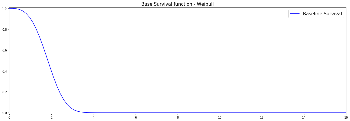
Pysurvival also displays the Base Survival function of the Simulation model:
from pysurvival.utils.display import display_baseline_simulations
display_baseline_simulations(sim, figure_size=(20, 6))

#### 3 - Creating the modeling dataset
# Defining the features
features = sim.features

# Building training and testing sets #
index_train, index_test = train_test_split( range(N), test_size = 0.2)
data_train = dataset.loc[index_train].reset_index( drop = True )
data_test  = dataset.loc[index_test].reset_index( drop = True )

# Creating the X, T and E input
X_train, X_test = data_train[features], data_test[features]
T_train, T_test = data_train['time'].values, data_test['time'].values
E_train, E_test = data_train['event'].values, data_test['event'].values

#### 4 - Creating an instance of the Linear MTLR model and fitting the data.
# Building the model
l_mtlr = LinearMultiTaskModel(bins=50)
l_mtlr.fit(X_train, T_train, E_train, lr=1e-3, init_method='orthogonal')


#### 5 - Cross Validation / Model Performances
c_index = concordance_index(l_mtlr, X_test, T_test, E_test) #0.95
print('C-index: {:.2f}'.format(c_index))

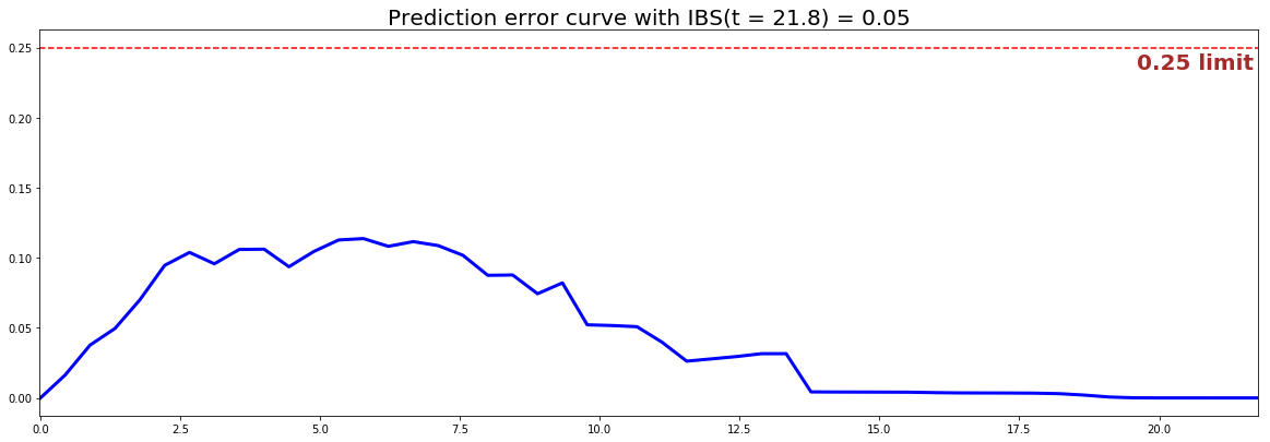
ibs = integrated_brier_score(l_mtlr, X_test, T_test, E_test, t_max=30,
            figure_size=(20, 6.5) )
print('IBS: {:.2f}'.format(ibs))
We can see that the c-index is well above 0.5 and that the Prediction error curve is below the 0.25 limit, thus the model yields great performances.

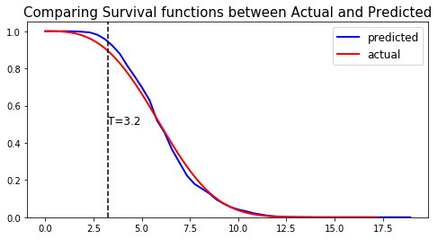
We can show this by randomly selecting datapoints and comparing the actual and predicted survival functions, computed by the simulation model and the Linear MTLR respectively.
#### 6 - Comparing actual and predictions
# Initializing the figure
fig, ax = plt.subplots(figsize=(8, 4))

# Randomly extracting a data-point that experienced an event
choices = np.argwhere((E_test==1.)&(T_test>=1)).flatten()
k = np.random.choice( choices, 1)[0]

# Saving the time of event
t = T_test[k]

# Computing the Survival function for all times t
predicted = l_mtlr.predict_survival(X_test.values[k, :]).flatten()
actual = sim.predict_survival(X_test.values[k, :]).flatten()

# Displaying the functions
plt.plot(l_mtlr.times, predicted, color='blue', label='predicted', lw=2)
plt.plot(sim.times, actual, color = 'red', label='actual', lw=2)

# Actual time
plt.axvline(x=t, color='black', ls ='--')
ax.annotate('T={:.1f}'.format(t), xy=(t, 0.5), xytext=(t, 0.5), fontsize=12)

# Show everything
title = "Comparing Survival functions between Actual and Predicted"
plt.legend(fontsize=12)
plt.title(title, fontsize=15)
plt.ylim(0, 1.05)
plt.show()
