

Predicting when your customers will churn

1 - Introduction

Customer churn/attrition, a.k.a the percentage of customers that stop using a company's products or services, is one of the most important metrics for a business, as it usually costs more to acquire new customers than it does to retain existing ones.

Indeed, according to a study by Bain & Company, existing customers tend to buy more from a company over time, thus reducing the operating costs of the business and may refer the products they use to others. For example, in financial services, a 5% increase in customer retention produces more than a 25% increase in profit.

By using Survival Analysis, not only companies can predict if customers are likely to stop doing business but also when that event might happen.

---

2 - Set up

A software as a service (SaaS) company provides a suite of products for Small-to-Medium enterprises, such as data storage, Accounting, Travel and Expenses management as well as Payroll management.

So as to help the CFO forecast the acquisition and marketing costs for the next fiscal year, the Data Science team wants to build a churn model to predict when customers are likely to stop their monthly subscription. Thus, once customers have been flagged as likely to churn within a certain time window, the company could take the necessary retention actions.

---

3 - Dataset

3.1 - Description and Overview

The dataset the team wants to use contains the following features:

Feature category	Feature name	Type	Description
Time	months_active	numerical	Number of months since the customer started his/her subscription
Event	churned	categorical	Specifies if the customer stopped doing business with the company
Products	product_data_storage	numerical	Amount of cloud data storage purchased in Gigabytes
Products	product_travel_expense	categorical	Indicates if the customer is actively using and paying for the Travel and Expense management services or not. ('Active', 'Free-Trial', 'No')
Products	product_payroll	categorical	Indicates if the customer is actively using and paying for the Payroll management services or not. ('Active', 'Free-Trial', 'No')
Products	product_accounting	categorical	Indicates if the customer is actively using and paying for the Accounting services or not. ('Active', 'Free-Trial', 'No')
Satisfaction	csat_score	numerical	Customer Satisfaction Score (CSAT) is the measure of how products and services supplied by the company meet customer expectations.
Satisfaction	minutes_customer_support	numerical	Minutes the customer spent on the phone with the company customer support
Marketing	articles_viewed	numerical	Number of articles the customer viewed on the company website.
Marketing	smartphone_notifications_viewed	numerical	Number of smartphone notifications the customer viewed
Marketing	marketing_emails_clicked	numerical	Number of marketing emails the customer opened on
Marketing	social_media_ads_viewed	numerical	Number of social media ads the customer viewed
Customer information	company_size	categorical	Size of the company
Customer information	us_region	categorical	Region of the US where the customer's headquarter is located

# Importing modules
import pandas as pd
import numpy as np
from matplotlib import pyplot as plt
from pysurvival.datasets import Dataset
%pylab inline

# Reading the dataset
raw_dataset = Dataset('churn').load()
print("The raw_dataset has the following shape: {}.".format(raw_dataset.shape))
raw_dataset.head(2)

Here is an overview of the raw dataset:

product_data_storage	csat_score	articles_viewed	...	churned
1024	9	2	...	0
2048	10	7	...	0

3.2 - From categorical to numerical

There are several categorical features that need to be encoded into one-hot vectors:

• product_travel_expense
• product_payroll
• product_accounting
• us_region
• company_size

# Creating one-hot vectors
categories = ['product_travel_expense', 'product_payroll', 'product_accounting',
              'us_region', 'company_size']
dataset = pd.get_dummies(raw_dataset, columns=categories, drop_first=True)

# Creating the time and event columns
time_column = 'months_active'
event_column = 'churned'

# Extracting the features
features = np.setdiff1d(dataset.columns, [time_column, event_column] ).tolist()

4 - Exploratory Data Analysis

As this tutorial is mainly designed to provide an example of how to use PySurvival, we will not do a thorough exploratory data analysis here but greatly encourage the reader to do so by checking the predictive maintenance tutorial that provides a detailed analysis.

Here, we will just check if the dataset contains Null values or if it has duplicated rows. Then, we will take a look at feature correlations.

4.1 - Null values and duplicates

The first thing to do is checking if the raw_dataset contains Null values and has duplicated rows.

# Checking for null values
N_null = sum(dataset[features].isnull().sum())
print("The raw_dataset contains {} null values".format(N_null)) #0 null values

# Removing duplicates if there exist
N_dupli = sum(dataset.duplicated(keep='first'))
dataset = dataset.drop_duplicates(keep='first').reset_index(drop=True)
print("The raw_dataset contains {} duplicates".format(N_dupli))

# Number of samples in the dataset
N = dataset.shape[0]

As it turns out the dataset doesn't have any Null values or duplicates.

4.2 - Correlations

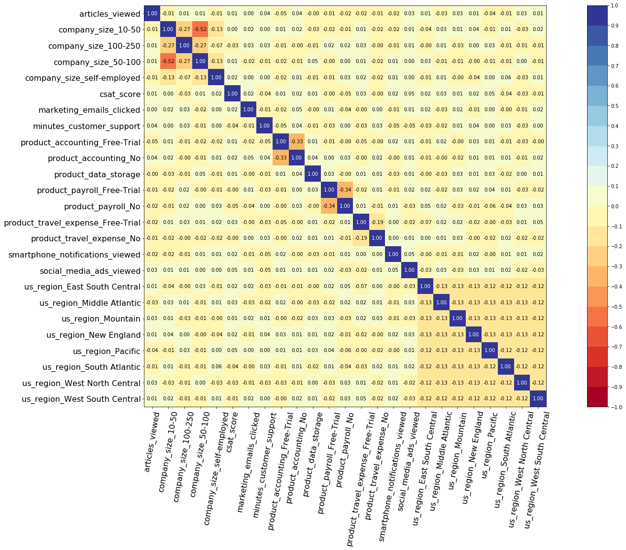
Let's compute and visualize the correlation between the features

from pysurvival.utils.display import correlation_matrix
correlation_matrix(dataset[features], figure_size=(30,15), text_fontsize=10)

Figure 1 - Correlations

As we can see, there aren't any alarming correlations.

---

5 - Modeling

5.1 - Building the model

So as to perform cross-validation later on and assess the performances of the model, let's split the dataset into training and testing sets.

# Building training and testing sets
from sklearn.model_selection import train_test_split
index_train, index_test = train_test_split( range(N), test_size = 0.35)
data_train = dataset.loc[index_train].reset_index( drop = True )
data_test  = dataset.loc[index_test].reset_index( drop = True )

# Creating the X, T and E inputs
X_train, X_test = data_train[features], data_test[features]
T_train, T_test = data_train[time_column], data_test[time_column]
E_train, E_test = data_train[event_column], data_test[event_column]

Let's now fit a Conditional Survival Forest model to the training set.

Note: The choice of the hyper-parameters was obtained using grid-search selection, not displayed in this tutorial.

from pysurvival.models.survival_forest import ConditionalSurvivalForestModel

# Fitting the model
csf = ConditionalSurvivalForestModel(num_trees=200)
csf.fit(X_train, T_train, E_train, max_features='sqrt',
        max_depth=5, min_node_size=20, alpha=0.05, minprop=0.1)

5.2 - Variables importance

Having built a Survival Forest model allows us to compute the features importance:

# Computing variables importance
csf.variable_importance_table.head(5)

Here is the top 5 of the most important features.

feature	importance	pct_importance
csat_score	11.251287	0.176027
product_payroll_No	11.204996	0.175303
minutes_customer_support	9.167136	0.143421
product_accounting_No	7.768278	0.121535
product_payroll_Free-Trial	3.669896	0.057416

Thanks to the feature importance, we get a better understanding of what drives retention or churn. Here, the Accounting and Payroll Management products, score on the satisfaction survey as well as the amount of time spent on the phone with customer support play a primordial role.

Note: The importance is the difference in prediction error between the perturbed and unperturbed error rate as depicted by Breiman et al.

---

6 - Cross Validation

In order to assess the model performance, we previously split the original dataset into training and testing sets, so that we can now compute its performance metrics on the testing set:

6.1 - C-index

The C-index represents the global assessment of the model discrimination power: this is the model’s ability to correctly provide a reliable ranking of the survival times based on the individual risk scores. In general, when the C-index is close to 1, the model has an almost perfect discriminatory power; but if it is close to 0.5, it has no ability to discriminate between low and high risk subjects.

from pysurvival.utils.metrics import concordance_index
c_index = concordance_index(csf, X_test, T_test, E_test)
print('C-index: {:.2f}'.format(c_index)) #0.83

6.2 - Brier Score

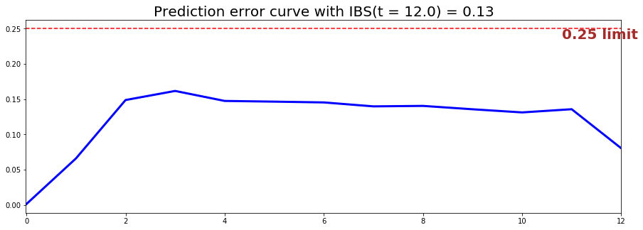
The Brier score measures the average discrepancies between the status and the estimated probabilities at a given time. Thus, the lower the score (usually below 0.25), the better the predictive performance. To assess the overall error measure across multiple time points, the Integrated Brier Score (IBS) is usually computed as well.

from pysurvival.utils.display import integrated_brier_score
ibs = integrated_brier_score(csf, X_test, T_test, E_test, t_max=12,
    figure_size=(15,5))
print('IBS: {:.2f}'.format(ibs))

Figure 2 - Conditional Survival Forest - Brier scores & Prediction error curve

The IBS is equal to 0.13 on the entire model time axis. This indicates that the model will have good predictive abilities.

---

7 - Predictions

7.1 - Overall predictions

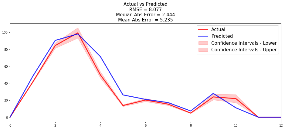
Now that we have built a model that seems to provide great performances, let's compare the time series of the actual and predicted number of customers who stop doing business with the SaaS company, for each time t.

from pysurvival.utils.display import compare_to_actual
results = compare_to_actual(csf, X_test, T_test, E_test,
                            is_at_risk = False,  figure_size=(16, 6),
                            metrics = ['rmse', 'mean', 'median'])

Figure 3 - Conditional Survival Forest - Number of customers who churned

The model provides very good results overall since on an entire 12 months window, it only makes an average absolute error of ~5 customers.

---

7.2 - Individual predictions

Now that we know that we can provide reliable predictions for an entire cohort, let's compute the probability of remaining a customer for all times t.

First, we can construct the risk groups based on risk scores distribution. The helper function create_risk_groups, which can be found in pysurvival.utils.display, will help us do that:

from pysurvival.utils.display import create_risk_groups

risk_groups = create_risk_groups(model=csf, X=X_test,
    use_log = False, num_bins=30, figure_size=(20, 4),
    low={'lower_bound':0, 'upper_bound':8.5, 'color':'red'},
    medium={'lower_bound':8.5, 'upper_bound':12.,'color':'green'},
    high={'lower_bound':12., 'upper_bound':25,  'color':'blue'}
    )

Figure 4 - Conditional Survival Forest - Risk groups

Note: The current choice of the lower and upper bounds for each group is based on my intuition; so feel free to change the values so as to match your situation instead.

---

Here, it is possible to distinguish 3 main groups, low, medium and high risk groups. Because the C-index is high, the model will be able to properly rank the survival time of random units of each group, such that $t_{high} \leq t_{medium} \leq t_{low}$.

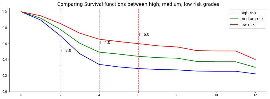
Let's randomly select individual unit in each group and compare their probability of remaining a customer for all times t. To demonstrate our point, we will purposely select units which experienced an event to visualize the actual time of event.

# Initializing the figure
fig, ax = plt.subplots(figsize=(15, 5))

# Selecting a random individual that experienced an event from each group
groups = []
for i, (label, (color, indexes)) in enumerate(risk_groups.items()) :

    # Selecting the individuals that belong to this group
    if len(indexes) == 0 :
        continue
    X = X_test.values[indexes, :]
    T = T_test.values[indexes]
    E = E_test.values[indexes]

    # Randomly extracting an individual that experienced an event
    choices = np.argwhere((E==1.)).flatten()
    if len(choices) == 0 :
        continue
    k = np.random.choice( choices, 1)[0]

    # Saving the time of event
    t = T[k]

    # Computing the Survival function for all times t
    survival = csf.predict_survival(X[k, :]).flatten()

    # Displaying the functions
    label_ = '{} risk'.format(label)
    plt.plot(csf.times, survival, color = color, label=label_, lw=2)
    groups.append(label)

    # Actual time
    plt.axvline(x=t, color=color, ls ='--')
    ax.annotate('T={:.1f}'.format(t), xy=(t, 0.5*(1.+0.2*i)),
        xytext=(t, 0.5*(1.+0.2*i)), fontsize=12)

# Show everything
groups_str = ', '.join(groups)
title = "Comparing Survival functions between {} risk grades".format(groups_str)
plt.legend(fontsize=12)
plt.title(title, fontsize=15)
plt.ylim(0, 1.05)
plt.show()

Figure 5 - Conditional Survival Forest - Predicting individual probability to remain a customer

Here we can see that the model manages to provide great prediction of the event time.

---

8 - Conclusion

We can now save our model so as to put it in production and score future customers.

# Let's now save our model
from pysurvival.utils import save_model
save_model(csf, '/Users/xxx/Desktop/churn_csf.zip')

In conclusion, we can see that it is possible to predict when customers will stop doing business with the company at different time points. The model will help the company be more pro-active when it comes to retaining their customers; and provide a better understanding of the reasons that drive churn.

---

References:

• Churn definition from hubspot.com
• Bain & Company - Prescription for cutting costs
• Random Forests. Machine Learning, 45(1), 5-32